electric field hockey

for the first level i was able to to get a goal with two charges

for level 2 i was able to get a goal with 3 positive charges

here we analyzed two particles with charge and how that affected direction

.

negative point particles electrical field where field points inward

positive point particle electric field radiating outward

two plates that are equidistant from each other creating a field that does not change in magnitude between plates

here we analyzed each situation and gave an explanation

this is the excel calculations of the electrical force that a bar exerts on a point particle. using the numbers we were able to come up with a graph of distance vs electrical field. we were able to see an inverse relationship between the two. we did this again however with the point particle above the bar at different angles. 

charge repulsion

The picture on the left shows how we set up the tape and when we touched opposite ends the tips of the tap attracted together showing how positive and negative charged items react to one another.

This is a summary of what we were able to observe from the tape experiment

recording the distance between two charged particles as they got closer together we were able to create a graph of a electrical force vs separation distance and saw a power graph where where this says that the electrical force approaches zero as distance increases. 

here we showed that coulombs law accounts for the inverse relationship between distance and force.

Diesel Cycle

This is my calculations for the Diesel cycle. Using the given information for pressure vs temperature we calculated the pressure, temperature, and volume at each point. using that we were able to find the heat transfer, work, change in internal energy, and change in entropy. using this we were able to configure the efficiency of the system to be 61%

Gas Cycles

Here we were able to analyze a PV diagram. Using points on the graph we found the change in internal energy of the system. using this we calculated the work and heat transfer energy from a point on the graph to the next point Where each transition had a different effect on the system.

Using active physics for heat capacity we were able to visually see how the gas particles reacted with increasing and decreasing pressure and volume. we found that the the total heat transfer minus the work equaled the total internal energy. Using various points at different temperatures we could come up with the constant pressure molar heat capacity of an ideal gas. 

This was our PV graph prediction of a mass on a syringe.

This was the experimental graph that was accumulated from the mass increasing and decreasing pressure. 

This is a Carnot cycle which we used as a problem to determine the values of pressure and volume at each point. using the pressures and volumes we calculated the heat transfer, work, and change in internal energy. 

fire syringe

video of our fire syringe. start video at 20 seconds to see flame. 

Fire syringe we used to calculate the final temperature of the gas as we push the syringe down. 

This is our calculations for final temperature of the gas where we measured the initial and final volume, initial temperature of the gas, and initial and final length the syringe travels. using what was measured we were able to calculate a value of 2590.6K. Our biggest uncertainty would come from the measurements of the radius of the inner tube and the distance the plunger travels through which would give us a larger uncertainty. 

This is the answers for the state variable and ideal gas law questions. 

playing with the isothermal process we go a non linear curve as shown showing that as volume increases pressure decreases at a non constant rate and vice-versa. 

volume vs temperature for a gas

This was our set up for the lab to determine the relationship between the temperture of the water relative to the volume of the plunger considering negligible friction between the walls of the plunger.

First we found the entire volume of the flask with the stopper to be 40.5cc to account for all the air within the system. then we lowered the flask into three different temperatures: hot, cold, and room temperature. During each temp there was a volume change within the plunger representing how the temp affected the volume of the gas. From the results we were able to retreive three data points to graph.

Using these data points we were able to create a graph where we see a linear relationship between volume and temperature. Using this line we obtained a linear function where the slope represents the ideal gas law constant.

thermal expansion

Thermal Expansion

For the Thermal expansion experiment this was the set-up where steam from the boiler was used to heat up the rod at one end. on the other end was a measuring device which calculated the length of expansion through a rotated angle.

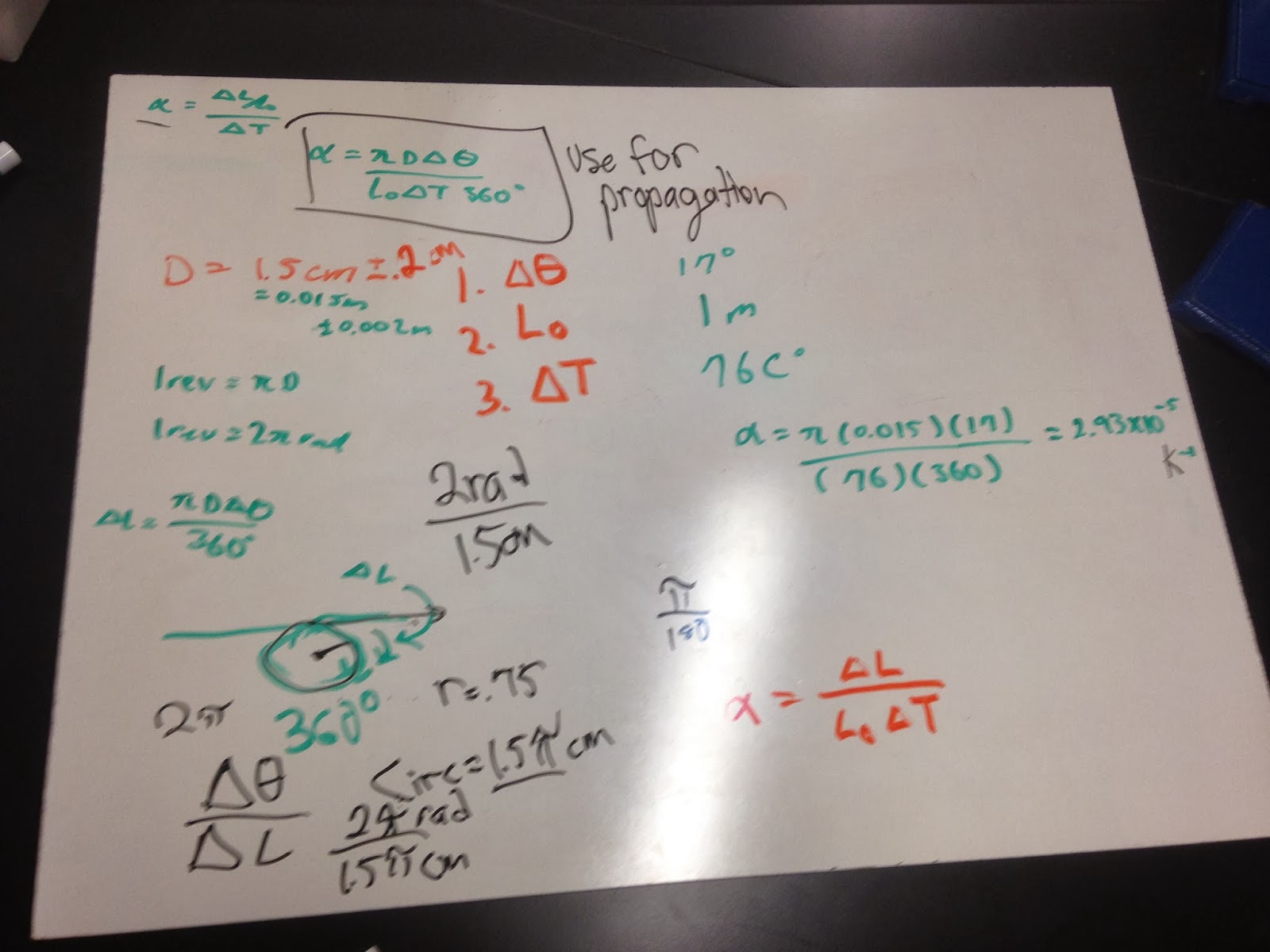
This is were we evaluated the expansion rate of a metal rod with steam used as a heating source. the expansion of the rod would then move along the circumfrence of a circular measuring device. From these results we were able to calculate the expansion rate of the rod leading us to the probrable material of the rod. 

using the uncertainty in the distance we were able to evaluate the uncertainty in the expansion rate of the rod using partial differentiation. using this we are able to cover our uncertainty in our answer which could have arised from the measurement of the distance the rod moved. 

this was the graphical results from the steaming of the rod. this showed how the rise in temperature expanded the rod at a linear rate.  

Latent heat of Vaporization

this is the set up of recording the boiling point of the water for a period of time to measure the amount of water evaporated in order to calculate the latent heat of vaporization. 

This is our graphical results where we measured the length of time the water was boiling. This shows how the temp of the water will increase until just below 100 degrees Celsius and stay at that temp until all the water turns into vapor. 

using the power, change in time and mass we were able to calculate the latent heat of vaporization for water. This did differ from the actual value of 2.2*10^6 because we did not take into account the water was evaporation as the temp was rising which would have gotten us closer to the actual value. 

Using excel I calculated the standard deviation of the classrooms results and found that our results varied greatly between the average. from this it is saying that our values fall from 1779300+_ 858363. this is a wide spread due to the out lire  that increased our standard deviation. 

This is our prediction of how pressure is inversely proportional to the volume so as the pressure increases the volume decreases.

when we tried this experiment we were able to prove the relationship graphically. the slope represents the number of moles of gas. 

This was the setup for the pressure vs volume where we used a syringe to apply pressure. 

This is where we showed the pressure vs temperature where we showed that there is a linear relationship between pressure and temperature. the meaning of the constant represents the universal gas law constant.

this is the graphical representation of the pressure vs temperature where we were able to obtain the slope of the graph which is close to the universal gas constant.